A17 Photometric Stereo

Photometric stereo is the technique of extracting shapes from shadow.
We can estimate the shape of the surface by capturing multiple images of the sources at different locations. The information about the surface will be coded in the shadings obtained from the images.

In this activity we are given synthetic images of a sphere illuminated by a point source located respectively at

V1 = {0.085832, 0.17365, 0.98106}
V2 = {0.085832, -0.17365, 0.98106}
V3 = {0.17365, 0, 0.98481}
V4 = {0.16318, -0.34202, 0.92542}.

The figure below shows the multiple images



The program that I used is

//// four synthetic images of a sphere
loadmatfile('C:\Documents and Settings\VIP\Desktop\186 a17\Photos.mat');
I(1,:) = I1(:)';
I(2,:) = I2(:)';
I(3,:) = I3(:)';
I(4,:) = I4(:)';

scf(1);
subplot(2,2,1);
imshow(I1,[]);
subplot(2,2,2);
imshow(I2,[]);
subplot(2,2,3);
imshow(I3,[]);
subplot(2,2,4);
imshow(I4,[]);


///// Light source locations
V1 = [0.085832 0.17365 0.98106];
V2 = [0.085832 -0.17365 0.98106];
V3 = [0.17365 0 0.98481];
V4 = [0.16318 -0.34202 0.92542];
V = [V1;V2;V3;V4];

//// eqn 10
g = inv((V')*V)*(V')*I;

//// eqn 11
//absg=abs(g);
absg = ((g(1,:).^2 + g(2,:).^2 + g(3,:).^2).^0.5);
n(1, :) = g(1,:)./(absg + 0.00000000000000001);
n(2, :) = g(2,:)./(absg + 0.00000000000000001);
n(3, :) = (g(3,:)./(absg +0.00000000000000001))+ 0.00000000000001;

////eqn 14
dfdx = -(n(1,:))./n(3,:);
dfdy = -(n(2,:))./n(3,:);

root=sqrt(length(absg))
dfdx = matrix(dfdx, [root,root]);
dfdy = matrix(dfdy, [root,root]);

//// eqn 15
z = cumsum(dfdx, 2) +cumsum(dfdy, 1);

scf(2);
plot3d(1:root, 1:root, z);

The reconstruction is

It shows a half hemisphere although there are some ridges due to the abrupt changes in the shading

In this activity, I give myself a grade of 10 since I was able to do the reconstruction.

A16 Artificial Neural Networks

Artificial neural networks are modeled after the way our brain works. Just like our brain, ANN’s most defining feature is its ability to learn through successive trainings. Training of an ANN is done by presenting to the network a set of input and target pairs. The network will then adapt its weights or strengths of connections between neurons so that the difference between the target and the network’s output will be minimized.

Among the applications of ANNs is pattern recognition. The training set will have the features-matrix as input and the classes as target.

Some of the network parameters that can be manipulated are

1. Number of hidden layers/ neurons in the hidden layer

- Bigger networks can generally solve more complicated problems. However care must also be taken to limit network size so that memorization can be avoided.

2. Epoch

- Time when all patterns in the data set have been presented to the network. The weights are adjusted after each epoch.

3. Learning rate

- May be set by trial and error.

We still use the features extracted from the two previous activities…

… and the code from Cole’s blog.

The results of the training and testing classification for different learning rates are listed below.

Correct classification would be 0 for strawberries and 1 for blueberries. Notice that for both training and testing classification the values that the neural network outputs are not exactly 0 or 1. The sample is just classified to the class that is nearer to its own value. As the learning rate is increased the classification goes closer to 0 and 1. The same also happens when we increase the number of epochs.

I give myself a grade of 10 because all the classifications were correct.

A15 Probabilistic Classification

In A14, we used Minimum Distance Classification. In this activity, we implement another kind of classification scheme, which is the linear discriminant analysis or LDA.

We have already done feature extraction in A14, so we only need to worry about LDA implementation.

In general, the probabilistic classification criterion is to minimize the total error of classification. That is it follows Bayes rule and assigns an object to the class with the highest conditional probability. So if for example

then object x will be classified to class i.

Most of the time, however, it is easier to find out the probability that a class will have a particular feature vector than the probability that the feature vector belongs to a class. These two quantities are related by the Bayes theorem.

where P(i) is the prior probability or the probability about the group i that is known without making any measurement. In practice we can assume the prior probability is equal for all groups or based on the number of sample in each group.

In practice, however, this implementation requires lots of data. Instead we just assume a distribution and get the probability that an object belongs to a certain class from there. Assuming that each class has a multivariate Normal distribution and all classes have the same covariance matrix, gives us the Linear Discriminant Analysis formula:

where object to group that has maximum

LDA assumes that the classes are linearly separable. (This is ok, since the plots from a14 show that the features are indeed linearly separable.) The classes can then be separated by a linear combination of features that describe the objects. A feature vector with only 2 elements will have a separator that is a line. Three features will be separated by a plane and more than three features will be separated by a hyperplane.

The actual implementation is as follows. We used the features extracted from A14.


n1=3;n2=3; //number of test elements for fruit1 and fruit2

////////the training set features in matrix form with objects as rows and features as columns x1=[perim1(1:3,:) mr1(1:3,:) mb1(1:3,:)];
x2=[perim2(1:3,:) mr2(1:3,:) mb2(1:3,:)];
x_all=[x1;x2];

/////// classification of the training set
y=[1;1;1;1;1;1;2;2;2;2;2;2];

////// mean features
mean1=mean(x1,1);
mean2=mean(x2,1);
mean_all=mean([x1;x2],1);/// global mean vector


/////mean corrected data (data - global mean vector)
mean_corr1=x1-ones(n1,1)*mean_all;
mean_corr2=x2-ones(n2,1)*mean_all;


///covariance matrix
c1=mean_corr1'*mean_corr1/n1;
c2=mean_corr2'*mean_corr2/n2;


//// Pooled covariance matrix
C=[];
[r,s]=size(c1);
for i=1:r
for j=1:s
C(i,j)=(n1*c1(i,j) + n2*c2(i,j))/(n1+n2);
end end

invC=inv(C);

////prior probability
p=[n1;n2]./(n1+n2);


//// Discriminant function
f1=mean1*invC*x_all' - 0.5*mean1*invC*mean1' + log(p(1));
f2=mean2*invC*x_all' - 0.5*mean2*invC*mean2' + log(p(2));
classify=1*((f1-f2)<0)+1;


////////////////////////// Testing

/////// the testing set
//ordered
//x_predict=[perim1(4:6,:) mr1(4:6,:) mb1(4:6,:); perim2(4:6,:) mr2(4:6,:) mb2(4:6,:)];
//alternating
x_predict=[perim1(4,:) mr1(4,:) mb1(4,:); perim2(4,:) mr2(4,:) mb2(4,:);perim1(5,:) mr1(5,:) mb1(5,:); perim2(5,:) mr2(5,:) mb2(5,:);perim1(6,:) mr1(6,:) mb1(6,:); perim2(6,:) mr2(6,:) mb2(6,:)];

f1_predict=mean1*invC*x_predict' - 0.5*mean1*invC*mean1' + log(p(1)); f2_predict=mean2*invC*x_predict' - 0.5*mean2*invC*mean2' + log(p(2));
classify_predict=1*((f1_predict-f2_predict)<0)+1;

The results are summarized in the following tables.

TRAINING



All the training objects are classified correctly. There are zero errors in training.
We can now use the computed separator for the testing of objects not used in training.

TESTING

100% accuracy of classification. I give myself a grade of 10. =)

Reference:
http://people.revoledu.com/kardi/tutorial/LDA/LDA.html#LDA

A14 Pattern Recognition

In this activity, our task was to use image processing techniques in implementing pattern recognition. The task can actually be divided into two parts; first is the feature extraction and then the training and actual classification.

Let us first define some terms that are commonly used in pattern recognition.

Pattern - set of features

Features -quantifiable properties such as color, shape, size, etc.

Feature vector - ordered set of features

Class - a set of patterns that share common properties

For this activity, I chose to work with two classes of fruits: strawberries and blueberries.
There were 6 samples for each class. Of these, 3 will be used as a training set while the other 3 will be for independent testing. The images of the fruits are shown below.

FRUIT 1: Strawberry


FRUIT 2: Blueberry


PART 1: Feature Extraction

The features that I decided to extract were color ( as rg and also as RGB), perimeter and area.

First I had to separate the fruits from the background, so I used histogram backprojection (A12).
However the segmentation wasn't clean enough so I made use of my knowledge of opening and closing operations to fix it. Then I used follow() and bwlabel() to tag each sample. For each sample I then obtained the perimeter, area, perimeter-area ratio, rg and RGB.
The program that I used was as follows.

//// fruit 1 = strawberry
//// fruit 2 = blueberry
path = 'C:\Documents and Settings\2004-49537\Desktop\186 act14\';
img1 = imread(path+'fruits1.bmp');
objpatch1 = imread(path+'patch1.bmp');
imgseg1 = 1*(segment(img1,objpatch1)>0);
//scf(1); clf(1);
//imshow(imgseg1);
img2 = imread(path+'fruits2.bmp');
objpatch2 = imread(path+'patch2b.bmp');
imgseg2 = 1*(segment(img2,objpatch2)>0);
//scf(2); clf(2);
//imshow(imgseg2);
//// perform closing and opening
se1=[ 0 1 0 ; 1 1 1 ; 0 1 0 ]; se2=ones(7,5);
imgseg1=dilate(imgseg1,se2);
imgseg1=erode(imgseg1,se2);
imgseg1=erode(imgseg1,se1);
imgseg1=dilate(imgseg1,se1);
//scf(3); clf(3);
//imshow(imgseg1);
imgseg2=dilate(imgseg2,se2);
imgseg2=erode(imgseg2,se2);
imgseg2=erode(imgseg2,se1);
imgseg2=dilate(imgseg2,se1);
//scf(4); clf(4);
//imshow(imgseg2);
[L1,n1]=bwlabel(imgseg1);
[L2,n2]=bwlabel(imgseg2);
R1=img1(:,:,1);
G1=img1(:,:,2);
B1=img1(:,:,3);
I1=R1+G1+B1;
r1=R1./I1;
g1=G1./I1;
R2=img2(:,:,1);
G2=img2(:,:,2);
B2=img2(:,:,3);
I2=R2+G2+B2;
r2=R2./I2;
g2=G2./I2;

for i=1:n1

////// area
area1(i,:)=sum(sum(1*(L1==i)));
area2(i,:)=sum(sum(1*(L2==i)));

//// perimeter
perim1(i,:)=perim(1*(L1==i));
perim2(i,:)=perim(1*(L2==i));

////// color
[row1,col1]=find(L1==i);
[row2,col2]=find(L2==i);

for j=1:length(row1)
red1=[red1; R1(row1(j),col1(j))];
green1=[green1; G1(row1(j),col1(j))];
blue1=[blue1; B1(row1(j),col1(j))];
end

for j=1:length(row2)
red2=[red2; R2(row2(j),col2(j))];
green2=[green2; G2(row2(j),col2(j))];
blue2=[blue2; B2(row2(j),col2(j))];
end

mr1(i,:)=mean(red1);
mg1(i,:)=mean(green1);
mb1(i,:)=mean(blue1);
mr2(i,:)=mean(red2);
mg2(i,:)=mean(green2);
mb2(i,:)=mean(blue2);
end

apratio1=area1./perim1;
apratio2=area2./perim2;

where segment was a function that does histogram backprojection segmentation.

PART 2. Class Representative Vector

For each class, we used features from the first three samples to get the mean feature per class.

Noting that the greatest difference of mean features for the two classes and the least standard deviation of feature values within a class occurred for the perimeter, R, and B; I used these three to make up the mean feature vector per class.


The program is as follows.

/////// mean features
meanarea1=mean(area1(1:3,:));
meanarea2=mean(area2(1:3,:));
meanperim1=mean(perim1(1:3,:));
meanperim2=mean(perim2(1:3,:));
meanapratio1=mean(apratio1(1:3,:));
meanapratio2=mean(apratio2(1:3,:));
meanr1=mean(mr1(1:3,:));
meanr2=mean(mr2(1:3,:));
meanb1=mean(mb1(1:3,:));
meanb2=mean(mb2(1:3,:));

m1=[meanperim1 meanr1 meanb1]';
m2=[meanperim2 meanr2 meanb2]';

PART 3: Minimum Distance Classification

Class membership is then determined by assigning an object to the class that has a minimum euclidian distance from it in terms of the feature vectors. Or alternatively, we can compute

where x is the unknown object's feature vector and m sub j is the mean feature vector of class j.

The object will then be classified to the larger d


d1=x'*m1 - 0.5*m1'*m1;
d2=x'*m2 - 0.5*m2'*m2;

classify=1*((d1-d2)<0)+1;

The first testing set consists of 3 strawberries (fruit 1) and then three blueberries (fruit 2).
The classification is 100% correct.


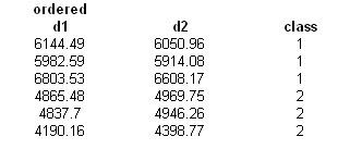
The second testing set consists of alternating strawberries (fruit 1) and blueberries (fruit 2).
The classification is still 100% correct.

Plotting in feature space, we see that...
(Red = fruit1; Green = fruit2; Circles = unknown class features; Star = mean features)

R vs B


Perimeter vs R

Perimeter vs B
The features of the two classes are clearly separable.

For this activity, I give myself a grade of 10. My classifications are 100% accurate.

Image from:
http://img2.allposters.com/images/NIM/KE041.jpg

A13 Correcting Geometric Distortion

Geometric distortions may result from the camera lens being spherical. Two common distortions are the barrel and the pin cushion distortions.

In barrel distortion, the image seems bloated in the middle and pinched at the sides.

The opposite happens for pin cushion distortion.

In this activity, we will try to correct pin cushion and barrel distortions.

First we need an image of a regularly repeating pattern like a grid or checkerboard as reference.
This will help us visualize the distortion that happens across the image.

Below, we show such a pattern for the barrel distortion

and for the pincushion distortion

Now, what we need to find is the transformation that will map the distorted image to the ideal image.

First we look at the transformation of pixel coordinates.

We assume that the coordinates are transformed in both directions simultaneously, so that r and s would be bilinear functions

The distorted coordinates would therefore be given by
To find the eight unknown coefficients c1-c8, we use the 4 vertices of a grid. These coefficients are valid only for points within the gird used and must therefore be generated for each grid in the image.

Using the four vertices, and rewriting the eight equations in matrix form we have
The distorted coordinates are easy to find. In Scilab, we just use the locate() function.
For the barrel distortion image above, the located points are marked with red crosses

Similarly for the pincushion
The ideal coordinates on the other hand are generated from the grid length down and across a grid from the most undistorted portion of the image (optical axis of the camera). In my program, I used

////count number of pixels down and across one box
//// choose diagonal points (origin and 1,1)
scf(1); clf();
imshow(im);
xy=locate(2,1);
//// ideal vertices
xoyo=xy(:,1);
xideal=(xoyo(1) + [-cols/2:cols/2]*xratio);
yideal=sort(xoyo(2) + [-rows/2:rows/2]*yratio);
a=ones(1:cols+3);
b=ones(1:rows+3);
xi=a'*xideal;
yi=yideal'*b;

where xi and yi are matrices that contain the column and row values of the grid vertices respectively. For example xi(1,2) will give the column value of the vertex at topmost row and 2nd to the left column.

We now know both the ideal and distorted vertices.

For the succeeding parts, I will place my discussions inside the code using comments.
(Its rather hard to discuss it step by step since they are all inside common loops)


/// The 2 for loops go through each grid
for i=1:rows
for j=1:cols

///Now to compute the 8 coefficients for each grid, I made the following code.
//// Computation of Coefficients per grid
T=[xi(i,j) yi(i,j) xi(i,j)*yi(i,j) 1; xi(i+1,j) yi(i+1,j) xi(i+1,j)*yi(i+1,j) 1; xi(i+1,j+1) yi(i+1,j+1)xi(i+1,j+1)*yi(i+1,j+1) 1; xi(i,j+1) yi(i,j+1) xi(i,j+1)*yi(i,j+1) 1];
Xd=([xd(i,j) xd(i+1,j) xd(i+1,j+1) xd(i,j+1)])';
Yd=([yd(i,j) yd(i+1,j) yd(i+1,j+1) yd(i,j+1)])';
C1_4=inv(T)*Xd;
C5_8=inv(T)*Yd;
c=[C1_4;C5_8];

//// The vertices of the ideal grid are given by
Xi=([xi(i,j) xi(i+1,j) xi(i+1,j+1) xi(i,j+1)])';
Yi=([yi(i,j) yi(i+1,j) yi(i+1,j+1) yi(i,j+1)])';
xir=floor(Xi); yir=floor(Yi);


//Now we go through each pixel in the grid.
for l=min(yir):max(yir)-1
for m=min(xir):max(xir)-1

//Per pixel in the ideal grid the location of that point in the distorted image is given by
xdistort2=c(1)*m + c(2)*l + c(3)*m.*l + c(4);
ydistort2=c(5)*m + c(6)*l + c(7)*m.*l + c(8);
xdr2=floor(xdistort2);
ydr2=floor(ydistort2);

////// Gray Level Interpolation
// ////The final part of the problem is to find the gray level value at the ideal pixel location.
//////This should just be a matter of assigning to the ideal coordinates the pixel value at the corresponding //////distorted coordinates (calculated using the two equations above).
//////However, the two equations above would not give exact integers all the time and so we need to //////interpolate the graylevel value. The interpolation that will be done here is the bilinear interpolation, //////whereas the gray level value at (x,y) is given by

////// a b c d can be obtained from the four nearest pixels of the location rather like the way we calculated the //////unknown coefficients c1-c4.
V=[im(ydr2,xdr2); im(ydr2+1,xdr2); im(ydr2,xdr2+1); im(ydr2+1,xdr2+1)];
Tv=[xdr2 ydr2 xdr2*ydr2 1; xdr2 (ydr2+1) xdr2*(ydr2+1) 1; (xdr2+1) ydr2 (xdr2+1)*ydr2 1; (xdr2 +1) (ydr2 +1) (xdr2 +1)*(ydr2+1) 1];
abcd=inv(Tv)*V;
im2(l,m)=(abcd(1)*xdistort2 +abcd(2)*ydistort2 + abcd(3)*xdistort2.*ydistort2 + abcd(4));

end
end

end
end

After correction the barrel distorted image now looks like (only the center 4 rows and columns)

while the pin cushion image looks like (only the center 4 rows and columns)

I also tried correcting distortions on more complicated images, like the cd rack below

and here is the result




Alternately, undistorted images can be distorted using the same procedure. We just have to superimpose a distorted pattern over an undistorted image, apply correction to the lines and voila! The image becomes distorted.

For this activity, I give myself a grade of 10. I was able to implement the correction for the barrel and pincushion distortion.

Images from
http://www.astrosurf.com/buil/iris/tutorial19
Ref
Activity 13 Manual

A12 Color Image Segmentation

In this activity, we color segment an image using parametric and non parametric segmentation.

For the non parametric segmentation, we did histogram backprojection wherein based on a color histogram of the ROI a pixel location is given a value equal to its histogram value in chromaticity space.

The parametric segmentation was done by assuming a gaussian pdf independently along r and g values of the ROI.

Since we are using 2D histograms, we first check if we are indeed getting the right colors.
Here the cropped portion is blue. Comparing our histogram with the chromaticity diagram below, we can see that the histogram is indeed correct. (I rotated the axis of the chromaticity so as to coincide with the histogram origin whichis at the upperleft corner.)


The results for the two methods are shown below.

A. Mugs

The image is


The cropped ROI is


For the non parametric segmentation, the result is



while for the parametric segmentation







B. Obama Lantern
The portion that I cropped is the light yellow part.

The result for the nonparametric was
For the parametric the pdf and the segmented image are


C. Starry Starry Night

The image is


The cropped color is
The non parametric segmentation result is


The parametric segmentation pdf and result is

We can see that the parametric segmentation is a lot stricter than the non-paramertic segmentation. Parametric would work better for when we want to segment shades of colors that are very much alike. For less stricter segmentations use non parametric.

In this activity, I give myself a grade of 10 because I understood and was able to do everything that was required.