A14 Pattern Recognition

In this activity, our task was to use image processing techniques in implementing pattern recognition. The task can actually be divided into two parts; first is the feature extraction and then the training and actual classification.

Let us first define some terms that are commonly used in pattern recognition.

Pattern - set of features

Features -quantifiable properties such as color, shape, size, etc.

Feature vector - ordered set of features

Class - a set of patterns that share common properties

For this activity, I chose to work with two classes of fruits: strawberries and blueberries.
There were 6 samples for each class. Of these, 3 will be used as a training set while the other 3 will be for independent testing. The images of the fruits are shown below.

FRUIT 1: Strawberry


FRUIT 2: Blueberry


PART 1: Feature Extraction

The features that I decided to extract were color ( as rg and also as RGB), perimeter and area.

First I had to separate the fruits from the background, so I used histogram backprojection (A12).
However the segmentation wasn't clean enough so I made use of my knowledge of opening and closing operations to fix it. Then I used follow() and bwlabel() to tag each sample. For each sample I then obtained the perimeter, area, perimeter-area ratio, rg and RGB.
The program that I used was as follows.

//// fruit 1 = strawberry
//// fruit 2 = blueberry
path = 'C:\Documents and Settings\2004-49537\Desktop\186 act14\';
img1 = imread(path+'fruits1.bmp');
objpatch1 = imread(path+'patch1.bmp');
imgseg1 = 1*(segment(img1,objpatch1)>0);
//scf(1); clf(1);
//imshow(imgseg1);
img2 = imread(path+'fruits2.bmp');
objpatch2 = imread(path+'patch2b.bmp');
imgseg2 = 1*(segment(img2,objpatch2)>0);
//scf(2); clf(2);
//imshow(imgseg2);
//// perform closing and opening
se1=[ 0 1 0 ; 1 1 1 ; 0 1 0 ]; se2=ones(7,5);
imgseg1=dilate(imgseg1,se2);
imgseg1=erode(imgseg1,se2);
imgseg1=erode(imgseg1,se1);
imgseg1=dilate(imgseg1,se1);
//scf(3); clf(3);
//imshow(imgseg1);
imgseg2=dilate(imgseg2,se2);
imgseg2=erode(imgseg2,se2);
imgseg2=erode(imgseg2,se1);
imgseg2=dilate(imgseg2,se1);
//scf(4); clf(4);
//imshow(imgseg2);
[L1,n1]=bwlabel(imgseg1);
[L2,n2]=bwlabel(imgseg2);
R1=img1(:,:,1);
G1=img1(:,:,2);
B1=img1(:,:,3);
I1=R1+G1+B1;
r1=R1./I1;
g1=G1./I1;
R2=img2(:,:,1);
G2=img2(:,:,2);
B2=img2(:,:,3);
I2=R2+G2+B2;
r2=R2./I2;
g2=G2./I2;

for i=1:n1

////// area
area1(i,:)=sum(sum(1*(L1==i)));
area2(i,:)=sum(sum(1*(L2==i)));

//// perimeter
perim1(i,:)=perim(1*(L1==i));
perim2(i,:)=perim(1*(L2==i));

////// color
[row1,col1]=find(L1==i);
[row2,col2]=find(L2==i);

for j=1:length(row1)
red1=[red1; R1(row1(j),col1(j))];
green1=[green1; G1(row1(j),col1(j))];
blue1=[blue1; B1(row1(j),col1(j))];
end

for j=1:length(row2)
red2=[red2; R2(row2(j),col2(j))];
green2=[green2; G2(row2(j),col2(j))];
blue2=[blue2; B2(row2(j),col2(j))];
end

mr1(i,:)=mean(red1);
mg1(i,:)=mean(green1);
mb1(i,:)=mean(blue1);
mr2(i,:)=mean(red2);
mg2(i,:)=mean(green2);
mb2(i,:)=mean(blue2);
end

apratio1=area1./perim1;
apratio2=area2./perim2;

where segment was a function that does histogram backprojection segmentation.

PART 2. Class Representative Vector

For each class, we used features from the first three samples to get the mean feature per class.

Noting that the greatest difference of mean features for the two classes and the least standard deviation of feature values within a class occurred for the perimeter, R, and B; I used these three to make up the mean feature vector per class.


The program is as follows.

/////// mean features
meanarea1=mean(area1(1:3,:));
meanarea2=mean(area2(1:3,:));
meanperim1=mean(perim1(1:3,:));
meanperim2=mean(perim2(1:3,:));
meanapratio1=mean(apratio1(1:3,:));
meanapratio2=mean(apratio2(1:3,:));
meanr1=mean(mr1(1:3,:));
meanr2=mean(mr2(1:3,:));
meanb1=mean(mb1(1:3,:));
meanb2=mean(mb2(1:3,:));

m1=[meanperim1 meanr1 meanb1]';
m2=[meanperim2 meanr2 meanb2]';

PART 3: Minimum Distance Classification

Class membership is then determined by assigning an object to the class that has a minimum euclidian distance from it in terms of the feature vectors. Or alternatively, we can compute

where x is the unknown object's feature vector and m sub j is the mean feature vector of class j.

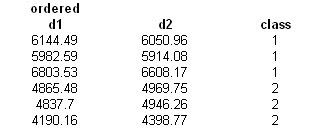
The object will then be classified to the larger d


d1=x'*m1 - 0.5*m1'*m1;
d2=x'*m2 - 0.5*m2'*m2;

classify=1*((d1-d2)<0)+1;

The first testing set consists of 3 strawberries (fruit 1) and then three blueberries (fruit 2).
The classification is 100% correct.


The second testing set consists of alternating strawberries (fruit 1) and blueberries (fruit 2).
The classification is still 100% correct.

Plotting in feature space, we see that...
(Red = fruit1; Green = fruit2; Circles = unknown class features; Star = mean features)

R vs B


Perimeter vs R

Perimeter vs B
The features of the two classes are clearly separable.

For this activity, I give myself a grade of 10. My classifications are 100% accurate.

Image from:
http://img2.allposters.com/images/NIM/KE041.jpg